OSPF on Packet Tracer

We are going to apply OSPF(open shortest path first) protocol on packet tracer. Let us take the following simple topology.



Now, let us apply the ospf on it. But before that, as usual :) , let us assign IP addresses and change the state of interfaces.

 

Similarly for the other router.

Lab Manual Of Computer Communication and Networks

1	Introduction to Networking Devices	https://cs-study.blogspot.com/2012/09/networking-devices.html
2	Introduction to Packet Tracer	https://cs-study.blogspot.com/2012/10/what-is-packet-tracer.html
3	Packet Tracer CLI commands	https://cs-study.blogspot.com/2012/10/packet-tracer-cli.html
4	Introduction to Cables	https://cs-study.blogspot.com/2012/10/networking-cables-and-connections.html
5	Communication in PT, getting started ..	https://cs-study.blogspot.com/2012/10/communication-between-pcs-in-packet.html
6	RIP on Packet Tracer	https://cs-study.blogspot.com/2012/10/rip-on-packet-tracer.html
7	RIP V2 on Packet Tracer	https://cs-study.blogspot.com/2012/10/rip-version-2-on-packet-tracer.html
8	EIGRP on Packet Tracer	https://cs-study.blogspot.com/2012/10/eigrp-on-packet-tracer.html
9	OSPF on Packet Tracer	https://cs-study.blogspot.com/2013/03/ospf-on-packet-tracer.html
10	DHCP on Router	https://cs-study.blogspot.com/2012/10/dhcp-on-packet-tracer.html
11	DHCP on PT through Server	https://cs-study.blogspot.com/2012/10/dhcp-on-packet-tracer-through-server.html
12	DNS on Packet Tracer	https://cs-study.blogspot.com/2012/10/dns-on-packet-tracer.html
13	VLANS on Packet Tracer	https://cs-study.blogspot.com/2012/11/vlan-on-packet-tracer.html
14	VTP on Packet Tracer	https://cs-study.blogspot.com/2012/11/vtp-on-packet-tracer.html
15	Spanning Tree Protocol on Packet Tracer	https://cs-study.blogspot.com/2012/11/spanning-tree-protocol-on-packet-tracer.html
16	Sticky MAC addresses	https://cs-study.blogspot.com/2012/12/sticky-mac-addresses.html
17	Inter VLAN Routing (Router on a Stick)	https://cs-study.blogspot.com/2012/11/inter-vlan-routing-router-on-stick.html
18	CDP on Packet Tracer	https://cs-study.blogspot.com/2012/12/cdp-cisco-discovery-protocol.html
19	Telnet and SSH	https://cs-study.blogspot.com/2012/12/telnet-and-ssh-on-packet-tracer.html
20	Password Authentication Protocol on PT	https://cs-study.blogspot.com/2012/12/password-authentication-protocol-on.html
21	Challenge Hand Shake Authentication Protocol on PT	https://cs-study.blogspot.com/2012/12/point-to-point-protocol-on-packet.html
22	Voice Over IP on PT (VOIP)	https://cs-study.blogspot.com/2012/12/voice-over-ip-voip-on-packet-tracer.html
23	Wireless Communication on Packet Tracer	https://cs-study.blogspot.com/2012/12/wireless-communication-in-packet-tracer.html
24	Access Control List on PT	https://cs-study.blogspot.com/2012/11/acl-on-packet-tracer.html
	NS2 (Network Simulator - 2) Tutorials
25	NS 2 and Ubuntu Installation	https://cs-study.blogspot.com/2012/12/ns2-installation-and-ubuntu.html
26	Nodes Creation in NS 2	https://cs-study.blogspot.com/2012/12/add-following-code-to-new-file-and.html
27	Traffic Flow in NS 2	https://cs-study.blogspot.com/2012/12/traffic-flow-on-nodes-in-ns2.html
28	Dynamic Nodes generation and traffic flow in ns2	https://cs-study.blogspot.com/2013/05/dynamic-nodes-generation-and-traffic.html
29	Xgraph in NS2	https://cs-study.blogspot.com/2013/05/xgraph-in-ns2.html

 30   Wireless Communication in NS2

Technorati Tags: Lab Manual,Packet Tracer tutorial,Packet Tracer lab manual,Networking tutorial manual,NS 2 manual,network simulator installation manual

Quick Sort

 

Quicksort is another divide and conquer algorithm. Quicksort is based on the idea of partitioning (splitting) the list around a pivot or split value. Quicksort is also a divide and conquer algorithm. We see pictorially, how the quick sort algorithm works. Suppose we have an array as shown in the figure Fig 45.33.

We select an element from the array and call it the pivot. In this array, the pivot is the middle element 5 of the array. Now, we swap this with the last element 3 of the array. The updated figure of the array is shown in Fig 45.34.

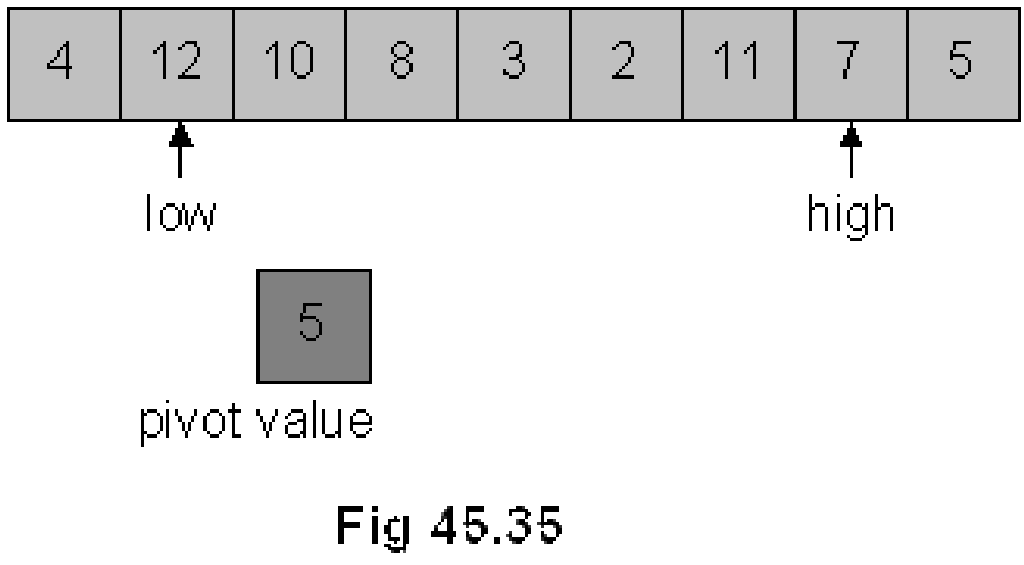
As shown in Fig 45.34, we used two indexes low and high. The index low is started from 0^th position of the array and goes towards right until n-1^th position. Inside this loop, an element that is bigger than the pivot is searched. The low index is incremented further as 4 is less than 5.

low is pointing to element 12 and it is stopped here as 12 is greater than 5. Now, we start from the other end, the high index is moved towards left from n-1^th position to 0. While coming from right to left, we search such an element that is smaller than 5. Elements 7 and 11 towards left are greater than 5, therefore, the high pointer is advanced further towards left. high index is stopped at the next position as next element 2 is smaller than 5. Following figure Fig 45.36 depicts the latest situation.

Divide and Conquer

We had started discussing three new sorting algorithms; merge sort, quick sort and heap sort. All of these three algorithms take time proportional to nlog₂n. Our elementary three sorting algorithms were taking n² time; therefore, these new algorithms with nlog₂n time are faster. In search operation, we were trying to reduce the time from n to log₂n.

Let’s discuss these sorting algorithms; merge sort, quick sort and heap sort in detail.

We had started our discussion from divide and conquer rule where we also saw an example. Instead of sorting a whole array, we will divide it in two parts, each part is sorted separately and then they are merged into a single array.

Let’ see few analysis to confirm the usefulness of the divide and conquer technique.

- To sort the halves approximate time is (n/2)2+(n/2)2

- To merge the two halves approximate time is n

- So, for n=100, divide and conquer takes approximately:

= (100/2)2 + (100/2)2 + 100

= 2500 + 2500 + 100

= 5100 (n2 = 10,000)

Comparison of Complexity of Algorithms

We have studied these three algorithms i.e. selection sort, insertion sort and bubble sort. Now considering the above three algorithms, we see that these algorithms are easy to understand. Coding for these algorithms is also easy. These three algorithms are in place algorithms. There is no need of extra storage for sorting an array by these algorithms. With respect to the time complexity, these algorithms are proportional to N². Here N is the number of elements. So we can see that as the value of N increases, the performance time of these algorithms increases considerably as it is proportional to N². Thus these algorithms are expensive with respect to time performance. There are algorithms that have the time complexity proportional to N log₂ (N). The following table shows the respective values of N² and N log₂(N) for some values of N.

N	N2	N Log2 (N)
10	100	33.21
100	10000	664.38
1000	1000000	9965.78
10000	100000000	132877.12
100000	10000000000	1660964.04
1000000	1E+12	19931568.57

From this table we can see that for a particular value of N, the value of N² is very large as compared to the value of N log₂ (N). Thus we see that the algorithms whose time complexity is proportional to N² are much time consuming as compared to the algorithms the time complexity of which is proportional to N log₂ (N). Thus we see that the N log₂ (N) algorithms are better than the N² algorithms.

N log₂ (N) Algorithms

Now let’s see the algorithms that are N log₂ (N) algorithms. These include the following algorithms.

• Merge Sort
• Quick Sort
• Heap Sort

These three algorithms fall under ‘divide and conquer category’. The divide and conquer strategy is well known in wars. The philosophy of this strategy is ,’ divide your enemy into parts and then conquer these parts’. To conquer these parts is easy, as these parts cannot resist or react like a big united enemy. The same philosophy is applied in the above algorithms. To understand the divide and conquer strategy in sorting algorithm, let’s consider an example. Suppose we have an unsorted array of numbers is given below.

Bubble Sort

The third sorting algorithm is bubble sort. The basic idea of this algorithm is that we bring the smaller elements upward in the array step by step and as a result, the larger elements go downward. If we think about array as a vertical one, we do bubble sort. The smaller elements come upward and the larger elements go downward in the array. Thus it seems a bubbling phenomenon. Due to this bubbling nature, this is called the bubble sort. Thus the basic idea is that the lighter bubbles (smaller numbers) rise to the top. This is for the sorting in ascending order. We can do this in the reverse order for the descending order.

The steps in the bubble sort can be described as below

• Exchange neighboring items until the largest item reaches the end of the array

• Repeat the above step for the rest of the array

In this sort algorithm, we do not search the array for the smallest number like in the other two algorithms. Also we do not insert the element by shifting the other elements. In this algorithm, we do pair-wise swapping. We will take first the elements and swap the smaller with the larger number. Then we do the swap between the next pair. By repeating this process, the larger number will be going to the end of the array and smaller elements come to the start of the array.

Insertion Sort

The main idea of insertion sort is

• Start by considering the first two elements of the array data. If found out of order, swap them

• Consider the third element; insert it into the proper position among the first three elements.

• Consider the fourth element; insert it into the proper position among the first four elements.

• … …

This algorithm is not something uncommon to the persons who know card playing. In the game of cards, a player gets 13 cards. He keeps them in the sorted order in his hand for his ease. A player looks at the first two cards, sorts them and keeps the smaller card first and then the second. Suppose that two cards were 9 and 8, the player swap them and keep 8 before 9. Now he takes the third card. Suppose, it is 10, then it is in its position. If this card is of number 2, the player will pick it up and put it on the start of the cards. Then he looks at the fourth card and inserts it in the first three cards (that he has sorted) at a proper place. He repeats the same process with all the cards and finally gets the cards in a sorted order. Thus in this algorithm, we keep the left part of the array sorted and take element from the right and insert it in the left part at its proper place. Due to this process of insertion, it is called insertion sorting.