November 17, 2012

Operations on Binary Tree

 
We can define different operations on binary trees.
If p is pointing to a node in an existing tree, then
  • left(p) returns pointer to the left subtree
  • right(p) returns pointer to right subtree
  • parent(p) returns the father of p
  • brother(p) returns brother of p.
info(p) returns content of the node
Consider a tree has been formed already, following methods will be used to perform different operations on a node of this tree:
Operation Description
left(p) Returns a pointer to the left sub-tree
right(p) Returns a pointer to the right sub-tree
parent(p) Returns the father node of p
brother(p) Returns the brother node of p
info(p) Returns the contents of node p
These methods have already been discussed at the end of the previous lecture, however, few more methods are required to construct a binary tree:
Operation Description
setLeft(p, x) Creates the left child node of p and set the value x into it.
setRight(p, x) Creates the right child node of p, the child node contains the info x.
All these methods are required to build and to retrieve values from a tree.
Applications of Binary Tree
Let’s take few examples to understand how the tree data type is used and what are its benefits. We will also develop some algorithms that may by useful in future while working with this data type.
Binary tree is useful structure when two-way decisions are made at each point. Suppose we want to find all duplicates in a list of the following numbers:
14, 15, 4, 9, 7, 18, 3, 5, 16, 4, 20, 17, 9, 14, 5
This list may comprise numbers of any nature. For example, roll numbers, telephone numbers or voter’s list. In addition to the presence of duplicate number, we may also require the frequency of numbers in the list. As it is a small list, so only a cursory view may reveal that there are some duplicate numbers present in this list. Practically, this list can be of very huge size ranging to thousands or millions.
Searching for Duplicates
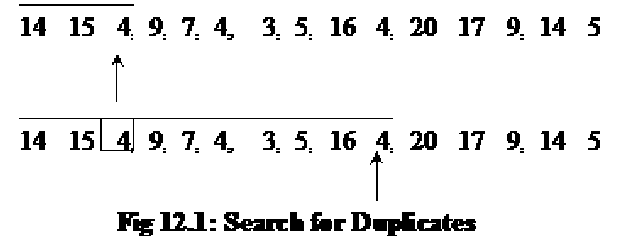
One way of finding duplicates is to compare each number with all those that precede it. Let’s see it in detail.
clip_image001
Suppose, we are looking for duplicates for the number 4, we will start scanning from the first number 14. While scanning, whenever we find the number 4 inside, we remember the position and increment its frequency counter by 1. This comparison will go on till the end of the list to get the duplicates or fequence of the number 4. You might have understood already that we will have to perform this whole scanning of list every time for each number to find duplicates. This is a long and time consuming process.
So this procedure involves a large number of comparisons, if the list of numbers is large and is growing.
A linked list can handle the growth. But it can be used where a programmer has no idea about the size of the data before hand. The number of comparisons may still be large. The comparisons are not reduced after using linked list as it is a linear data structure. To search a number in a linked list, we have to begin from the start of the list to the end in the linear fashion, traversing each node in it. For optimizing search operation in a list, there is no real benefit of using linked list. On the contrary, the search operation becomes slower even while searching in an array because the linked list is not contiguous like an array and traversing is done in the linked list with the help of pointers.
So, the solution lies in reducing the number of comparisons. The number of comparisons can be drastically reduced with the help of a binary tree. The benefits of linked list are there, also the tree grows dynamically like the linked list.
The binary tree is built in a special way. The first number in the list is placed in a node, designated as the root of the binary tree. Initially, both left and right sub-trees of the root are empty. We take the next number and compare it with the number placed in the root. If it is the same, this means the presence of a duplicate. Otherwise, we create a new tree node and put the new number in it. The new node is turned into the left child of the root node if the second number is less than the one in the root. The new node is turned into the right child if the number is greater than the one in the root.
clip_image002
In the above figure, the first number in the list 14 is placed in a node , making it the root of the binary tree. You can see that it is not pointing to any further node. Therefore, its left and right pointers are NULL at this point of tree construction time. Now, let’s see, how do we insert the next element into it.
clip_image003
As a first step to add a new node in the tree, we take the next number 15 in the list and compare it with 14, the number in the root node. As they are different, so a new node is created and the number 15 is set into it.
clip_image004
The next step is to add this node in the tree. We compare 15, the number in the new node with 14, the number in the root node. As number 15 is greater than number 14, therefore, it is placed as right child of the root node.
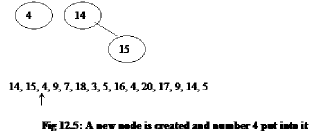
The next number in the list i.e. 4, is compared with 14, the number in the root node. As the number 4 is less than number 14, so we see if there is a left child of the root node to compare the number 4 with that. At this point of time in the tree, there is no further left child of the root node. Therefore, a new node is created and the number 4 is put into it.
The below figure shows the newly created node.
clip_image005
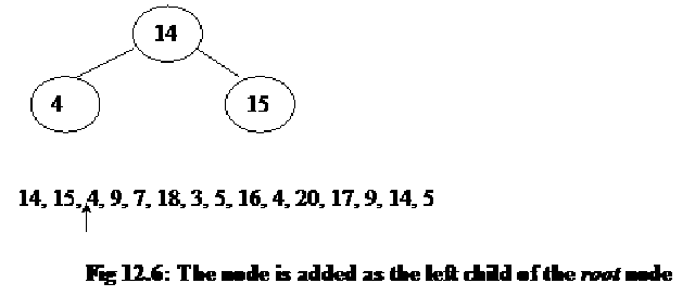
Next, the newly created node is added as the left child of the root node. It is shown in the figure below.
clip_image006
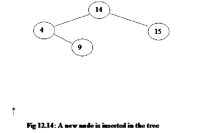
The next number in the list is 9. To add this number in the tree, we will follow the already defined and experimented procedure. We compare this number first with the number in the root node of the tree. This number is found to be smaller than the number in the root node. Therefore, left sub-tree of the root node is sought. The left child of the root node is the one with number 4. On comparison, number 9 is found greater than the number 4. Therefore, we go to the right child of the node with number 4. At the moment, there is no further node to the right of it, necessitating the need of creating a new node. The number 9 is put into it and the new node is added as the right child of the node with number 4. The same is shown in the figure given below.
clip_image007
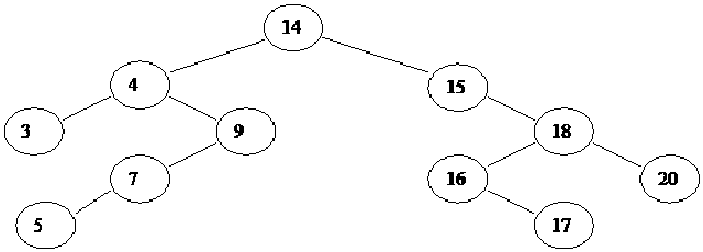
We keep on adding new nodes in the tree in line with the above practiced rule and eventually, we have the tree shown in the below figure.
clip_image008
clip_image009
 
It is pertinent to note that this is a binary tree with two sub-nodes or children of each node. We have not seen the advantage of binary tree, the one we were earlier talking about i.e. it will reduce the number of comparisons. Previously, we found that search operation becomes troublesome and slower as the size of list grows. We will see the benefit of using binary tree over linked list later. Firstly, we will see how the tree is implemented.
 

C++ Implementation of Binary Tree

See the code below for the file treenode.cpp.
/* This file contains the TreeNode class declaration. TreeNode contains the functionality for a binary tree node */
1. #include <stdlib.h>
2.
3. template <class Object>
4.
5. class TreeNode
6. {
7. public:
8. // constructors
9. TreeNode()
10. {
11. this->object = NULL;
12. this->left = this->right = NULL;
13. };
14.
15. TreeNode( Object * object )
16. {
17. this->object = object;
18. this->left = this->right = NULL;
19. };
20.
21. Object * getInfo()
22. {
23. return this->object;
24. };
25.
26. void setInfo(Object * object)
27. {
28. this->object = object;
29. };
30.
31. TreeNode * getLeft()
32. {
33. return left;
34. };
35.
36. void setLeft(TreeNode * left)
37. {
38. this->left = left;
39. };
40.
41 TreeNode * getRight()
42. {
43. return right;
44. };
45.
46. void setRight(TreeNode * right)
47. {
48. this->right = right;
49. };
50.
51. int isLeaf( )
52. {
53. if( this->left == NULL && this->right == NULL )
54. return 1;
55. return 0;
56. };
57.
58. private:
59. Object * object;
60. TreeNode * left;
61. TreeNode * right;
62. }; // end class TreeNode


For implementation, we normally write a class that becomes a factory for objects of that type. In this case too, we have created a class TreeNode to be used to create nodes of the binary tree. As we want to use this class for different data types, therefore, we will make it a template class, the line 2 is doing the same thing. Inside the class body, we start with the private data members given at the bottom of the class declaration. At line 59, the object is a private data element of Object *, used to store the tree element (value) inside the node of the tree. left is a private data member of type TreeNode*, it is used to store a pointer to the left sub-tree. right is a private data member of type TreeNode*, employed to store a pointer to the right sub-tree.
Now, we go to the top of the class declaration to see the public functions. At line 9, a public parameter-less constructor is declared. The data members have been initialized in the constructor. At line 11, the object data member is initialized to NULL. Similarly left and right data members are initialized to NULL at line 12.
There is another constructor declared at line 15- that takes object value as a parameter to construct a TreeNode object with that object value. While the pointers for right and left sub-trees are pointing to NULL.
At line 21, there is method getInfo(), which returns the object i.e. the element of the TreeNode object.
At line 26, the method setInfo(Object * ) sets the value of the object data member to the value passed to it as the argument.
The method getLeft() returns the pointer to the left sub-tree. Similarly, the getRight() returns the right sub-tree. Note that both of these methods return a pointer to the object of type TreeNode.
The setLeft(TreeNode *) method is used to set the pointer left to left sub-tree. Similarly, setRight(TreeNode *) is used to set the pointer right to right sub-tree. Both of these methods accept a pointer of type TreeNode.
The isLeaf() method at line 51, is to see whether the current node is a leaf node or not. The method returns 1 if it is leaf node. Otherwise, it returns 0.
Using the above TreeNode, nodes for the binary tree can be created and linked up together to form a binary tree. We can write a separate method or a class to carry out the node creation and insertion into tree.
Let’s use this class by writing couple of functions. Below is the code of main program file containing the main() and insert() functions.

1. #include <iostream>
2. #include <stdlib.h>
3. #include "TreeNode.cpp"
4.
5. int main(int argc, char * argv[])
6. {
7. int x[] = {14,15,4,9,7,18,3,5,16,4,20,17,9,14,5,-1};
8. TreeNode <int> * root = new TreeNode<int>();
9. root->setInfo( &x[0] );
10. for(int i = 1; x[i] > 0; i++ )
11. {
12. insert( root, &x[i] );
13. }
14. }
15.
16. void insert (TreeNode <int> * root, int * info)
17. {
18. TreeNode <int> * node = new TreeNode <int> (info);
19. TreeNode <int> * p, * q;
20. p = q = root;
21. while( *info != *(p->getInfo()) && q != NULL )
22. {
23. p = q;
24. if( *info < *(p->getInfo()) )
25. q = p->getLeft();
26. else
27. q = p->getRight();
28. }
29.
30. if( *info == *( p->getInfo() ) )
31. {
32. cout << "attempt to insert duplicate: " << *info << endl;
33. delete node;
34. }
35. else if( *info < *(p->getInfo()) )
36. p->setLeft( node );
37. else
38. p->setRight( node );
39. } // end of insert


We have used the same list of numbers for discussion in this lecture. It is given at line 7 in the code. It is the same, only the last number is –1. This is used as delimiter or marker to indicate that the list has finished.
At line 8, we are creating a new TreeNode object i.e. a root node as the name implies. This node will contain an int type element as evident from the syntax.
At line 9, the first number in the list is set into the root node. At line 10, the for loop is started, which is inserting all the elements of the list one by one in the tree with the use of the insert() function. Most of the time, this loop will be reading the input numbers from the users interactively or from a file. It it is Windows application then a form can by used to take input from the user. In this implementation, our objective is to insert numbers in the tree and see the duplicates, so hard coding the numbers within our program will serve the purpose.
The insert() method starts from line 16. It is accepting two parameters. The first parameter is pointer to a TreeNode object, containing a value of int type while second is the info that is an int *.
In the first line of the function, line 18, a new node has been by calling the parameterized constructor of the TreeNode class.
Then at line 19, two pointer variables p and q are declared.
In line 20, we are initializing variables p and q to the root node.
In line 21, the while loop is being started, inside the while loop we are checking the equality of the number inside the node (being pointed to by pointer p) with the number being passed. The control is entered into the loop, if both the numbers are not equal and q is not pointing to NULL. This while loop will be terminated if the numbers in the two nodes are equal or end of a sub-tree is reached.
At line 23 inside the loop, p is assigned the value of q.
At line 24 inside the loop, if the number inside the node is smaller than the number in the node pointed to by the pointer p. Then at line 25, we are getting the left sub-tree address (left) and assigning it to the pointer q.
Otherwise, if this not the case, means the number in the node to be inserted is not smaller than the number in the node pointed to by the pointer p. Then at line 27, the right sub-tree address is retrieved and assigned to pointer q.
At line 30, the comparison is made to see if the both the values are equal (number in the node to be inserted and the number inside the node pointed to by the pointer p). In case they are equal, it displays a message with the number informing that a duplicate number has been found. This also means that the upper while loop was terminated because of equality of the two numbers. In the line 33, the newly created node is deleted afterwards.
At line 35, we are checking if the number in the newly constructed node is less than the number in the node at the end of a sub-tree. If this is so then the newly constructed node is inserted to the left of the tree node. The insertion code is at line 36.
If the number in the newly constructed node is greater than the number in the tree node, the newly constructed node will be inserted to the right of the tree node as shown on line 38. To make it clearer, let’s see the same thing, the insert() method pictorially.
Trace of insert
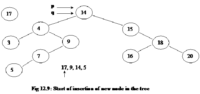
We will take the tree and the figure, we constructed above. At this time, we want to insert some new numbers in the tree as given in the figure below:
clip_image010
p
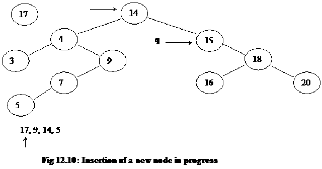
Initially the pointers p and q are pointing to the start (root) of the tree. We want to insert the number 17 in the tree. We compare the number in the root node (14) with number 17. Because number 17 is greater than the number 14, so as we did in the while loop in the function above, we will move toward the right sub-tree. In the next picture below, we can see that the pointer q has moved to the right sub-tree of the root.
clip_image011
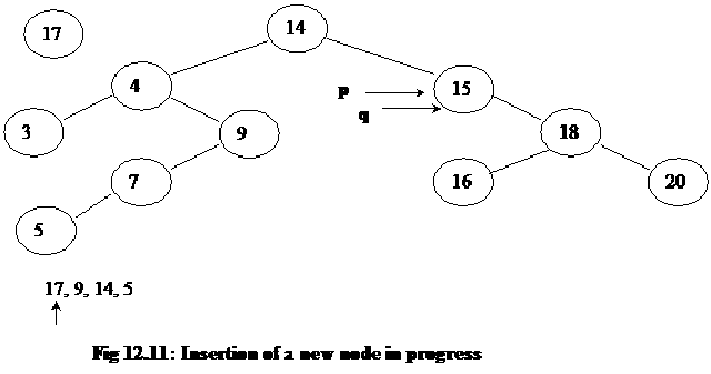
After moving the pointer q forward, we make the pointer p point to the same node. We do this operation as the first step inside the while loop. It can be seen at line 23 above. So following will be the latest position of pointers in the tree.
clip_image012
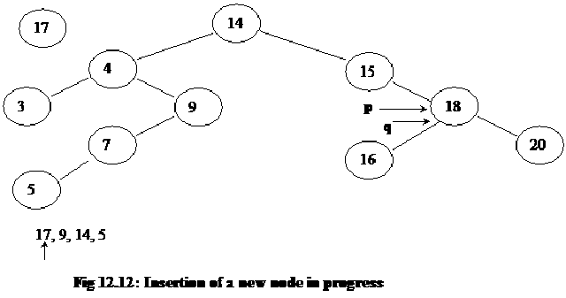
Now, the number 15 in the tree node is compared with new number 17. Therefore, the pointer q is again moved forward to the right child node i.e. the node with number 18. In the next step, we move forward the p pointer also. The following figure depicts the current picture of the tree:
clip_image013
The previous process is repeated again (while loop is the repeating construct) that the number 17 is compared with the number 18. This time the left child node is traversed and q pointer starts pointing the node with number 16 inside. In the next step, p is moved forward to point to the same node as q.
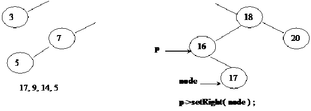
The same comparison process starts again, number 17 is found to be greater than the number 16, therefore, the right child is seek. But we see that the current tree node does not have right child node, so it returns NULL. Following figure depicts it.
clip_image014
clip_image015
Above shown (q is pointing to NULL) is the condition that causes the while loop in the code above to terminate. Later we insert the new node as the right child of the current node.
clip_image016
It is recommended to execute this algorithm manually to insert the remaining numbers in the tree. This will make the understanding more clear. This tree algorithm is going to be used rigorously in the future and complete understanding of it will make the complex future implementations easier to comprehend.

Trees and Binary Tree

This is an important data structure. This data structure is used in many algorithms. The data structures that we have discussed in previous lectures are linear data structures. The linked list and stack are linear data structures. In these structures, the elements are in a line. We put and get elements in and from a stack in linear order. Queue is also a linear data structure as a line is developed in it. There are a number of applications where linear data structures are not appropriate. In such cases, there is need of some non-linear data structure. Some examples will show us that why non-linear data structures are important. Tree is one of the non-linear data structures.
Look at the following figure. This figure (11.1) is showing a genealogy tree of a family.


In this genealogy tree, the node at the top of the tree is Grand Parent i.e. the head of the family. There are three nodes under this one. These are children of Grand Parent. Then there are nodes under these three nodes i.e. the children of these three family members. You may have seen the tree like this of some other family. You can make the tree of your family too. The thing to be noted in this genealogical tree is that it is not a linear structure like linked list, in which we have to tell that who is the father and who is the son. We make it like a tree. We develop the tree top-down, in which the father of the family is on the top with their children downward. We can see the similar tree structure of a company. In the tree of a company, the CEO of the company is on the top, followed downward by the managers and assistant managers. This process goes downward according to the administrative hierarchy of the company. Our tree structure is different from the actual tree in the way that the actual tree grows from down to up. It has root downside and the leaves upside. The data structure tree is opposite to the real tree as it goes upside down. This top-down structure in computer science makes it easy to understand the tree data structure.
There may be situations where the data, in our programs or applications, is not in the linear order. There is a relationship between the data that cannot be captured by a linked list or other linear data structure. Here we need a data structure like tree.
In some applications, the searching in linear data structures is very tedious. Suppose we want to search a name in a telephone directory having 100000 entries. If this directory is in a linked list manner, we will have to traverse the list from the starting position. We have to traverse on average half of the directory if we find a name. We may not find the required name in the entire directory despite traversing the whole list. Thus it would be better to use a data structure so that the search operation does not take a lot of time. Taking into account such applications, we will now talk about a special tree data structure, known as binary tree.
 Binary Tree
The mathematical definition of a binary tree is
“A binary tree is a finite set of elements that is either empty or is partitioned into three disjoint subsets. The first subset contains a single element called the root of the tree. The other two subsets are themselves binary trees called the left and right sub-trees”. Each element of a binary tree is called a node of the tree.
Following figure shows a binary tree.
clip_image003
Fig 11.2: A Binary Tree

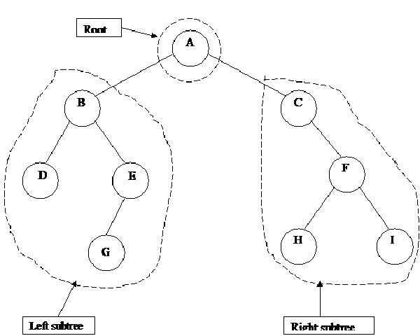
There are nine nodes in the above figure of the binary tree. The nine nodes are A, B, C, D, E, F, G, H, and I. The node A is at the top of the tree. There are two lines from the node A to left and right sides towards node B and C respectively. Let’s have a look at the left side of the node A. There are also two lines from node B to left and right, leading to the nodes D and E. Then from node, E there is only one line that is to the left of the node and leads to node G. Similarly there is a line from node C towards the node F on right side of the node C. Then there are two lines from node F that leads to the nodes H and I on left and right side respectively.
Now we analyze this tree according to the mathematical definition of the binary tree. The node A is the root of the tree. And tree structure (i.e. the nodes B, D, E, G and their relation) on the left side of the node A is a sub-tree, called the Left subtree. Similarly the nodes (C, F, H and I) on the right side of the node A comprise the sub-tree termed as Right subtree. Thus we made three parts of the tree. One part contains only one node i.e. A while the second part has all the nodes on left side of A, called as Left subtree. Similarly the third part is the Right subtree, containing the nodes on right side of A. The following figure depicts this scenario.
clip_image004

Fig 11.3: Analysis of a binary tree


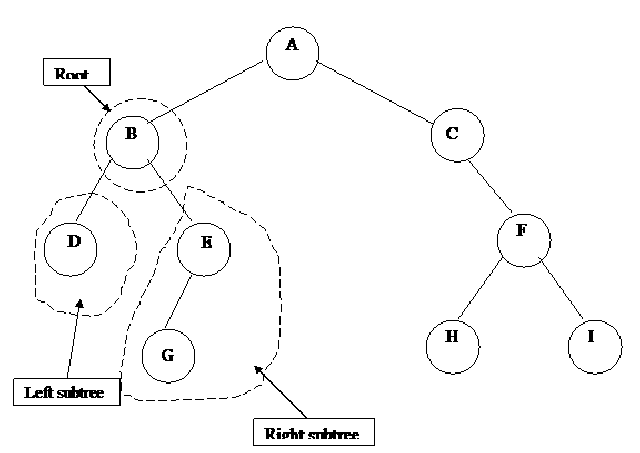
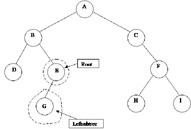
The same process of sub classing the tree can be done at the second level. That means the left and right subtrees can also be divided into three parts similarly. Now consider the left subtree of node A. This left subtree is also a tree. The node B is the root of this tree and its left subtree is the node D. There is only one node in this left subtree. The right subtree of the node B consists of two nodes i.e. E and G. The following figure shows the analysis of the tree with root B.
clip_image005
Fig 11.4: Analysis of a binary tree

On going one step down and considering right subtree of node B, we see that E is the root and its left subtree is the single node G. There is no right subtree of node E or we can say that its right subtree is empty. This is shown in the following figure.
clip_image006
Fig 11.5: Analysis of a binary tree

Now the left sub tree of E is the single node G. This node G can be considered as the root node with empty left and right sub trees. The definition of tree is of recursive nature. This is due to the fact that we have seen that which definition has been applied to the tree having node A as root, is applied to its subtrees one level downward. Similarly as long as we go down ward in the tree the same definition is used at each level of the tree. And we see three parts i.e. root, left subtree and right subtree at each level.

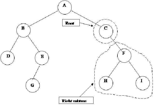
Now if we carry out the same process on the right subtree of root node A, the node C will become the root of this right subtree of A. The left subtree of this root node C is empty. The right subtree of C is made up of three nodes F, H and I. This is shown in the figure below.
clip_image007
Fig 11.6: Analysis of a binary tree

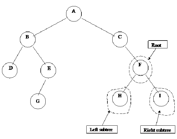
Now we apply the same recursive definition on the level below the node C. Now the right subtree of the node C will be considered as a tree. The root of this tree is the node F. The left and right subtrees of this root F are the nodes H and I respectively.
The following figure depicts this.
clip_image008
Fig 11.7: Analysis of a binary tree

We make (draw) a tree by joining different nodes with lines. But we cannot join any nodes whichever we want to each other. Consider the following figure.
clip_image009
Fig 11.8: A non-tree structure

It is the same tree, made earlier with a little modification. In this figure we join the node G with D. Now this is not a tree. It is due to the reason that in a tree there is always one path to go (from root) to a node. But in this figure, there are two paths (tracks) to go to node G. One path is from node A to B, then B to D and D to G. That means the path is A-B-D-G. We can also reach to node G by the other path that is the path A-B-E-G. If we have such a figure, then it is not a tree. Rather, it may be a graph. We will discuss about graphs at the end of this course.
Similarly if we put an extra link between the nodes A and B, as in the figure below, then it is also no more a tree. This is a multiple graph as there are multiple (more than 1) links between node A and B.
clip_image010
Fig 11.9: A non-tree structure

Similarly if we put other links between different nodes, then the structure thus developed will not be a tree. The following figure is also an example of a structure that is not a tree as there are multiple links between the different nodes.
clip_image011
Fig 11.10: A non-tree structure

Terminologies of a binary tree

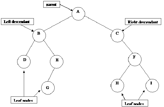
Now let’s discuss different terminologies of the binary tree. We will use these terminologies in our different algorithms. Consider the following figure.

clip_image012
Fig 11.11: Terminologies used in a binary tree

We have discussed that the node on the top is said root of the tree. If we consider the relationship of these nodes, A is the parent node with B and C as the left and right descendants respectively. C is the right descendant of A. Afterwards, we look at the node B where the node D is its left descendant and E is its right descendant. We can use the words descendant and child interchangeably. Now look at the nodes D, G, H and I. These nodes are said leaf nodes as there is no descendant of these nodes. We are just introducing the terminology here. In the algorithms, we can use the words root or parent, child or descendant. So the names never matter.

Strictly Binary Tree

There is a version of the binary tree, called strictly binary tree. A binary tree is said to be a strictly binary tree if every non-leaf node in a binary tree has non-empty left and right subtrees.
Now consider the previous figure 11.11. We know that a leaf node has no left or right child. Thus nodes D, G, H and I are the leaf nodes. The non-leaf nodes in this tree are A, B, C, E and F. Now according to the definition of strictly binary tree, these non-leaf nodes (i.e. A, B, C, E and F) must have left and right subtrees (Childs). The node A has left child B and right child C. The node B also has its left and right children that are D and E respectively. The non-leaf node C has right child F but not a left one. Now we add a left child of C that is node J. Here C also has its left and right children. The node F also has its left and right descendants, H and I respectively. Now the last non-leaf node E has its left child, G but no right one. We add a node K as the right child of the node E. Thus the tree becomes as shown below in the figure 11.12.
clip_image013
Fig 11.12: A Strictly binary tree

Now all the non-leaf nodes (A, B, C, E and F) have their left and right children so according to the definition, it is a strictly binary tree.
Level
The level of a node in a binary tree is defined as follows:
· Root has level 0,
· Level of any other node is one more than the level its parent (father).
· The depth of a binary tree is the maximum level of any leaf in the tree.
To understand level of a node, consider the following figure 11.13. This figure shows the same tree of figure 11.2, discussed so far.
clip_image014
0 ---------------------------------------- Level 0
1 1 ------------------- Level 1
2 2 2 ------- Level 2
3 3 3 -Level 3
Fig 11.13: Level of nodes of a tree

In the above figure, we have mentioned the level of each node. The figure also shows that the root node has level 0. We have talked in the definition of the level that the level of a node, other than root, is one more than the level of its parent. Now in the tree, the parent of nodes B and C is node A with level 0. Now by definition, the level of B and C will be 1 (i.e. level of A + 1). Now if go downward in the tree and see the nodes D, E and F, the parent node of D and E is B the level of which is 1. So the level of D and E is 2 (i.e. 1 + 1). Similarly the level of F is 2 as the level of its parent (i..e. C) is 1. In the same way, we can easily understand that the level of G, H and I is 3 as the parent nodes of these (E and F) have level 2. Thus we see that tree has multi levels in the downward direction. The levels of the tree increase, as the tree grows downward more. The number of nodes also increases.
Now let’s talk why we call it a binary tree. We have seen that each node has a maximum of two subtrees. There might be two, one or no subtree of a node. But it cannot have more than two. So, we call such a tree a binary one due to the fact that a node of it can have a maximum of two subtrees. There are trees whose nodes can have more than two subtrees. These are not binary trees. We will talk about these trees later.
By seeing the level of a tree, we can tell the depth of the tree. If we put level with each node of the binary tree, the depth of a binary tree is the maximum level. In the figure 11.13, the deepest node is at level 3 i.e. the maximum level is 3. So the depth of this binary tree is 3.

Complete Binary Tree
Now, if there are left and right subtrees for each node in the binary tree as shown below in figure 11.14, it becomes a complete binary tree.
clip_image015
0
1 1
2 2 2 2
3 3 3 3 3 3 3 3
Fig 11.14: A Complete Binary Tree

The definition of the complete binary tree is
“A complete binary tree of depth d is the strictly binary tree all of whose leaves are at level d”.
Now look at the tree, the leaf nodes of the tree are at level 3 and are H, I, J, K, L, M, N and O. There is no such a leaf node that is at some level other than the depth level d i.e. 3. All the leaf nodes of this tree are at level 3 (which is the depth of the tree i.e. d). So this is a complete binary tree. In the figure, all the nodes at level 3 are highlighted.
We know that the property of the binary tree is that its node can have a maximum of two subtrees, called as left and right subtrees. The nodes increase at each level, as the tree grows downward. In a complete binary tree, the nodes increase in a particular order. If we reconsider the previous tree (figure 11.14), we note that the number of node at level 0 is 1. We can say it 20, as 20 is equal to 1. Down to this, the node is the level 1 where the number of nodes is 2, which we can say 21, equal to 2. Now at the next level (i.e. level 2), the number of nodes is 4 that mean 22. Finally the number of nodes at level 3 is 8, which can be called as 23. This process is shown pictorially in the following figure 11.15.
clip_image017
------------- Level 0: 20 nodes
---------- Level 1: 21 nodes ----------
-------------- Level 2: 22 nodes -----------------
-
------------------------------------ Level 3: 23 nodes --------------------------------------------
Fig 11.15: Number of nodes at each level in a complete binary tree


By observing the number of nodes at a particular level, we come to the conclusion that the number of nodes at a level is equal to the level number raising to the power of two. Thus we can say that in a complete binary tree at a particular level k, the number of nodes is equal to 2k. Note that this formula for the number of nodes is for a complete binary tree only. It is not necessary that every binary tree fulfill this criterion. Applying this formula to each level while going to the depth of the tree (i.e. d), we can calculate the total number of nodes in a complete binary tree of depth d by adding the number of nodes at each level. This can be written as the following summation.
20+ 21+ 22 + ……… + 2d = Sd j=0 2j = 2d+1 – 1
Thus according to this summation, the total number of nodes in a complete binary tree of depth d will be 2d+1 – 1. Thus if there is a complete binary tree of depth 4, the total number of nodes in it will be calculated by putting the value of d equal to 4. It will be calculated as under.
24+1 - 1 = 25 – 1 = 32 – 1 = 31
Thus the total number of nodes in the complete binary tree of depth 4 is 31.
We know that the total number of nodes (leaf and non-leaf) of a complete binary tree of depth d is equal to 2d+1 – 1. In a complete binary tree, all the leaf nodes are at the depth level d. So the number of nodes at level d will be 2d . These are the leaf nodes. Thus the difference of total number of nodes and number of leaf nodes will give us the number of non-leaf (inner) nodes. It will be (2d+1 – 1) – 2d i.e. 2d – 1. Thus we conclude that in a complete binary tree, there are 2d leaf nodes and 2d – 1 non-leaf (inner) nodes.

Level of a Complete Binary Tree
We can conclude some more results from the above mathematical expression. We can find the depth of a complete binary tree if we know the total number of nodes. If we have a complete binary tree with n total nodes, then by the equation of the total number of nodes we can write
Total number of nodes = 2d+1 – 1 = n
To find the value of d, we solve the above equation as under
2d+1 – 1 = n
2d+1 = n + 1
d + 1 = log2 (n + 1)
d = log2 (n + 1) – 1
After having n total nodes, we can find the depth d of the tree by the above equation. Suppose we have 100,000 nodes. It means that the value of n is 100,000, reflecting a depth i.e. d of the tree will be log2 (100000 + 1) – 1, which evaluates to 20. So the depth of the tree will be 20. In other words, the tree will be 20 levels deep. The significance of all this discussion about the properties of complete binary tree will become evident later.

Uses of Queues

Out of the numerous uses of the queues, one of the most useful is simulation. A simulation program attempts to model a real-world phenomenon. Many popular video games are simulations, e.g., SimCity, Flight Simulator etc. Each object and action in the simulation has a counterpart in the real world. Computer simulation is very powerful tool and it is used in different high tech industries, especially in engineering projects. For example, it is used in aero plane manufacturing. Actually Computer Simulation is full-fledged subject of Computer Science and contains very complex Mathematics, sometimes. For example, simulation of computer networks, traffic networks etc.

If the simulation is accurate, the result of the program should mirror the results of the real-world event. Thus it is possible to understand what occurs in the real-world without actually observing its occurrence.
Let us look at an example. Suppose there is a bank with four tellers.
A customer enters the bank at a specific time (t1) desiring to conduct a transaction.
Any one of the four tellers can attend to the customer. The transaction (withdraws, deposit) will take a certain period of time (t2). If a teller is free, the teller can process the customer’s transaction immediately and the customer leaves the bank at t1+t2. It is possible that none of the four tellers is free in which case there is a line of customers at each teller. An arriving customer proceeds to the back of the shortest line and waits for his turn. The customer leaves the bank at t2 time units after reaching the front of the line.
The time spent at the bank is t2 plus time waiting in line.
So what we want to simulate is the working environment of the bank that there are specific number of queues of customers in the bank in front of the tellers. The tellers are serving customers one by one. A customer has to wait for a certain period of time before he gets served and by using simulation tool, we want to know the average waiting time of a bank customer. We will talk about this simulation in the next lecture and will do coding also in order to understand it well.
Suppose, customers want to deposit or withdraw money from a bank, having four cashiers or tellers. The teller helps you in depositing the money or withdrawing the money from the same window. This window is known as teller window. The customer needs some service from the bank like depositing the money, bill etc. This transaction needs some time that may be few minutes. A person enters the bank and goes to the teller who is free and requests him to do the job. After the completion of the transaction, the person goes out of the bank. Now we will discuss a scenario when there is a lot of rush of customers. The tellers are just four. Now the tellers are busy and the new customers will form a queue. In this example, we need a queue in front of each of the tellers. A new customer enters the bank and analyzes the four queues and wants to join the shortest queue. This person has to wait for the persons in front of him to be served. Another person may come behind him. In this simulation, we will restrict the person from changing the queue. A person comes into the bank at 10 O clock. His transaction time is 5 minutes. He has to wait for another fifteen minutes in the queue. After this, the teller serves him in 5 min. This person comes at 10 am and waits for fifteen minutes. As the transaction time is 5 minutes, so he will leave the bank at 1020. Now this is the situation of simulation and we have to write a program for this. We can go to some bank and analyze this situation and calculate the time. At the end of the day, we can calculate the average time for each of the customer. This time can be 30 minutes. Here we will simulate this situation with the help of a computer program. This is the real life example. Let’s see the picture of simulations to understand what is happening in the bank.
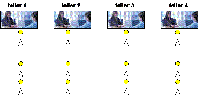
In the picture below, we have four tellers and four queues, one for each of the tellers. Each teller is serving a customer. When the transaction of a customer is completed, he will leave the bank.
clip_image002
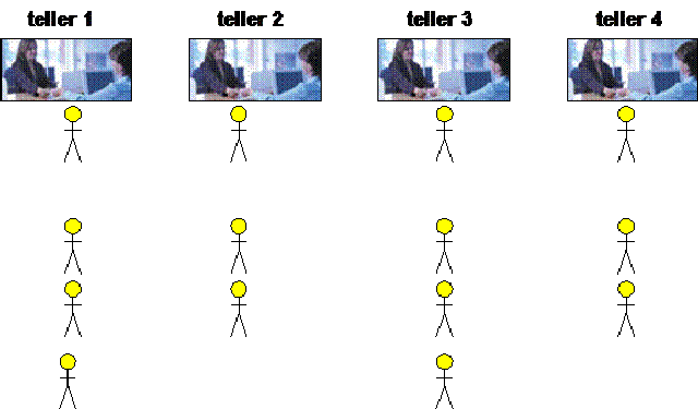
A person enters the bank. He sees that all the four tellers are busy and in each queue there are two persons waiting for their turn. This person chooses the queue no. 3. Another person enters the bank. He analyzed all the queues. The queue no 3 is the biggest and all other are having 2 persons in the queue. He chooses the queue no 1.
clip_image003
Now we have three persons waiting in queue no 1 and 3 and two persons waiting in queue no 2 and 4. The person in queue no.1 completes his transaction and leaves the bank. So the person in the front of the queue no. 1 goes to the teller and starts his transaction. Similarly the person at queue No. 3 finishes his transaction and leaves the premises. The person in front of queue number 3 goes to the teller.
Another person enters the bank and goes to the queue No. 1. This activity goes on. The queues become bigger and shorter. The persons coming in the bank have to wait. If the queues are shorter, people have to wait for less time. However, if the queues are longer, people have to wait for more time. The transactions can also take much more time, keeping the people waiting. Suppose four persons come with big amount and their transaction takes too much time. These are all parameters which we can incorporate in our simulation making it real. For this, we have carry out more programming. With the introduction of these parameters in the simulation, it will be more close to the real life situation. Simulation, being a very powerful technique, can yield the results, very close to some real life phenomenon.
Simulation Models
Let’s discuss little bit about the simulation models. Two common models of simulation are time-based simulation and event-based simulation. In time-based simulation, we maintain a timeline or a clock. The clock ticks and things happen when the time reaches the moment of an event.
Suppose we have a clock in the computer. The minute hand moves after every minute. We know the time of the customer’s entry into the bank and are aware that his transaction takes 5 minutes. The clock is ticking and after 5 minutes, we will ask the customer to leave the bank. In the program, we will represent the person with some object. As the clock continues ticking, we will treat all the customers in this way. Note that when the customer goes to some teller, he will take 5 minutes for his transaction. During this time, the clock keeps on ticking. The program will do nothing during this time period. Although some other customer can enter the bank. In this model, the clock will be ticking during the transaction time and no other activity will take place during this time. If the program is in some loop, it will do nothing in that loop until the completion of the transaction time.
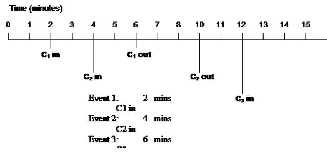
Now consider the bank example. All tellers are free. Customer C1 comes in 2 minutes after the opening of the bank. Suppose that bank opens at 9:00 am and the customer arrives at 9:02 am. His transaction (withdraw money) will require 4 minutes. Customer C2 arrives 4 minutes after the bank opens (9:04 am). He needs 6 minutes for transaction. Customer C3 arrives 12 minutes after the bank opens and needs 10 minutes for his transaction.
We have a time line and marks for every min.
clip_image004clip_image005
C1 comes at 2 min, C2 enters at 4 min. As C1 needs 4 min for his transaction, so he leaves at 6 min. C2 requires 6 min for the processing so C2 leaves at 10 min. Then C3 enters at 12 min and so on. This way, the activity goes on. Therefore, we can write a routine of the clock. We take a variable clock representing the clock. The clock will run for 24 hrs. Banks are not open for 24 hrs but we will run our loop for 24 hrs. The pseudo code is as under:
clock = 0;
while ( clock <= 24*60 ) { // one day
read new customer;
if customer.arrivaltime == clock
insert into shortest queue;
check the customer at head of all four queues.
if transaction is over
remove from queue.
clock = clock + 1;
}

The variable clock is initialized to zero. The while loop runs for 24 hrs. Then we read a new customer. This information may be coming from some file. The if statement is checking the arrival time of the customer. He comes 10 minutes after the opening of the bank. So when this time is equal to the clock, we insert the customer in the shortest queue. Then we will check the transaction time of all the four customers at each teller. If the transaction time of any customer ends, we will remove it from the queue and he will leave the bank. In the end, we increment the clock with one minute. As seen in the above statements, some activity takes place when the clock reaches at the event time (that is the time to enter the bank or leave the bank arrives). If the customer’s arrival time has not come, the first if statement becomes false and we do nothing. Similarly if the transaction of customer is not finished, the second if statement becomes false. Then this while loop will simply add one min to the clock. This is the clock- based (time- based) simulation.
Let’s discuss the other type of simulation i.e. the event-based simulation. Don’t wait for the clock to tick until the next event. Compute the time of next event and maintain a list of events in increasing order of time. Remove an event from the list in a loop and process it. Let’s see the time line again.
clip_image006clip_image007
The customer C1 comes at 2 min and leaves at 6 min. Customer C2 comes at 4 min and leaves at 10 min and so on. We have written the events list in the above figure. Do not see the clock but see the events on time. Event 1 occurs at 2 min that is the customer C1 enters the bank 2 minutes after its opening. Event 2 is that C2 enters at 4 min. Event 3 is that the customer C1 leaves the bank at 6 min. Event 4 is that the C2 leaves the bank at 10 min and event 5 is that C3 enters the bank at 12 min. Here we have a list of events. How can we process them? We will make a queue of these events. Remove the event with the earliest time from the queue and process it. Insert the newly created events in the queue. A queue where the de-queue operation depends not on FIFO, is called a priority queue.

Priority Queue

 The queue is a FIFO (First in first out) structure. In daily life, you have also seen that it is not true that a person, who comes first, leaves first from the queue. Let’s take the example of traffic. Traffic is stopped at the signal. The vehicles are in a queue. When the signal turns green, vehicles starts moving. The vehicles which are at the front of the queue will cross the crossing first. Suppose an ambulance comes from behind. Here ambulance should be given priority. It will bypass the queue and cross the intersection. Sometimes, we have queues that are not FIFO i.e. the person who comes first may not leave first. We can develop such queues in which the condition for leaving the queue is not to enter first. There may be some priority. Here we will also see the events of future like the customer is coming at what time and leaving at what time. We will arrange all these events and insert them in a priority queue. We will develop the queue in such a way that we will get the event which is going to happen first of all in the future. This data structure is known as priority queue. In a sense, FIFO is a special case of priority queue in which priority is given to the time of arrival. That means the person who comes first has the higher priority while the one who comes later, has the low priority. You will see the priority queue being used at many places especially in the operating systems. In operating systems, we have queue of different processes. If some process comes with higher priority, it will be processed first. Here we have seen a variation of queue. We will use the priority queue in the simulation. The events will be inserted in the queue and the event going to occur first in future, will be popped.

What are the requirements to develop this simulation? We need the C++ code for the simulation. There will be a need of the queue data structure and obviously, the priority queue. Information about the arrival of the customers will be placed in an input file. Each line of the file contains the items (arrival time, transaction duration).
Here are a few lines from the input file.
00 30 10 <- customer 1
00 35 05 <- customer 2
00 40 08
00 45 02
00 50 05
00 55 12
01 00 13
01 01 09


The first line shows the customer 1. “00 30 10” means Customer 1 arrives 30 minutes after the opening of the bank. He will need 10 minutes for his transaction. The last entry “01 01 09” means customer arrives one hour and one minute after the bank opened and his transaction will take 9 minutes and so on. The file contains similar information about the other customers. We will collect the events now. The first event to occur is the arrival of the first customer. This event is placed in the priority queue. Initially, the four teller queues are empty. The simulation proceeds as follows: when an arrival event is removed from the priority queue, a node representing the customer is placed on the shortest teller queue. Here we are trying to develop an algorithm while maintaining the events queue.
After the opening of the bank, the arrival of the first customer is the first event. When he enters the bank all the four tellers are free. Suppose he goes to the first teller and starts his transaction. After the conclusion of his transaction, he leaves the bank. With respect to events, we have only two events, one is at what time he enters the bank and other is at what time he leaves the bank. When other customers arrive, we have to maintain their events.
If the customer is the only one on a teller queue, an event for his departure is placed on the priority queue. At the same time, the next input line is read and an arrival event is placed in the priority queue. When a departure event is removed from the event priority queue, the customer node is removed from the teller queue. Here we are dealing with the events, not with the clock. When we come to know that a person is coming at say 9:20am, we make an event object and place it in the priority queue. Similarly if we know the time of leaving of the customer from the bank, we will make an event and insert it into the priority queue. When the next customer in the queue is served by the teller, a departure event is placed on the event priority queue. When the other customer arrives, we make an event object and insert it into the priority queue. Now the events are generated and inserted when the customer arrives. But the de-queue is not in the same fashion. When we de-queue, we will get the event which is going to occur first.
When a customer leaves the bank, the total time is computed. The total time spent by the customer is the time spent in the queue waiting and the time taken for the transaction. This time is added to the total time spent by all customers. At the end of the simulation, this total time divided by the total customers served will be average time consumed by customers. Suppose that 300 customers were served, then we will divide the total time by 300 to get the average time. So with the help of simulation technique, we will get the result that x customers came today and spent y time in the bank and the average time spent by a customer is z.

 Code of the Bank Simulation

Let’s have a look on the C+ code of this simulation.
#include <iostream>
#include <string>
#include <strstream.h>
#include "Customer.cpp"
#include "Queue.h"
#include "PriorityQueue.cpp"
#include "Event.cpp"
Queue q[4]; // teller queues
PriorityQueue pq; //eventList;
int totalTime;
int count = 0;
int customerNo = 0;
main (int argc, char *argv[])
{
Customer* c;
Event* nextEvent;
// open customer arrival file
ifstream data("customer.dat", ios::in);
// initialize with the first arriving customer.
ReadNewCustomer(data);
While( pq.length() > 0 )
{
nextEvent = pq.remove();
c = nextEvent->getCustomer();
if( c->getStatus() == -1 ){ // arrival event
int arrTime = nextEvent->getEventTime();
int duration = c->getTransactionDuration();
int customerNo = c->getCustomerNumber();
processArrival(data, customerNo,
arrTime, duration , nextEvent);
}
else { // departure event
int qindex = c->getStatus();
int departTime = nextEvent->getEventTime();
processDeparture(qindex, departTime, nextEvent);
}
}


We have included lot of files in the program. Other than the standard libraries, we have Customer.cpp, Queue.h, PriorityQueue.cpp and Event.cpp. With the help of these four files, we will create Customer object, Queue object, PriorityQueue object and Event object. You may think that these are four factories, creating objects for us.
As there are four tellers, so we will create equal number of queues (Queue q[4]). Then we create a priority queue object pq from the PriorityQueue factory. We declare totalTime, count and customerNo as int. These are global variables.
In the main method, we declare some local variables of customer and event. Afterwards, the customer.dat file for the input data is opened as:
ifstream data("customer.dat", ios::in);
We read the first customers data from this file as:
readNewCustomer(data);
Here data is the input file stream associated to customer.dat. We will read the arrival time and time of transaction from the file of the first customer. After reading it, we will process this information.
Now there is the while loop i.e. the main driver loop. It will run the simulation. First thing to note is that it is not clock-based which is that the loop will execute for 24 hours. Here we have the condition of priority queue’s length. The variable pq represents the event queue. If there are some events to be processed, the queue pq will not be empty. Its length will not be zero. We get the next event from the priority queue, not from the queue. The method pq.remove() (de-queue method) will give us the event which is going to happen first in future. The priority of events is according the time. In the event object we have the customerNo. In the if statement, we check the status of the customer. If the status is –1, it will reflect that this is the new customer arrival event.
We know that when a new customer enters the bank, he will look at the four tellers and go to the teller where the queue is smallest. Therefore in the program, we will check which is the smallest queue and insert the customer in that queue. If the event is about the new customer, the if statement returns true. We will get its arrival time, duration and customer number and assign it to the variables arrTime, duration and customerNo respectively. We will call the method processArrival() and pass it the above information.
If the status of the customer is not equal to –1, it means that the customer is in one of the four queues. The control will go to else part. We will get the status of the customer which can be 0, 1, 2 and 3. Assign this value to qindex. Later on, we will see how these values are assigned to the status. We will get the departure time of the customer and call the processDeparture() method.
In the main driver loop, we will get the next event from the event queue. In this case, events can be of two types i.e. arrival event and the departure event. When the person enters the bank, it is the arrival event. If any queue is empty, he will go to the teller. Otherwise, he will wait in the queue. After the completion of the transaction, the customer will leave the bank. It is the departure event.
Let’s discuss the function readNewCustomer(). This function is used to read the data from the file.
void readNewCustomer(ifstream& data)
{
int hour,min,duration;
if (data >> hour >> min >> duration) {
customerNo++;
Customer* c = new Customer(customerNo,
hour*60+min, duration);
c->setStatus( -1 ); // new arrival
Event* e = new Event(c, hour*60+min );
pq.insert( e ); // insert the arrival event
}
else {
data.close(); // close customer file
}
}


Here, we have used the >> to read the hour, minute and duration from the file. Then we create a customer object c from the customer factory with the new keyword. We pass the customerNo, arrival time and transaction duration to the constructor of the customer object. After the object creation, it is time to set its status to –1. This means that it is an arriving customer. Then we create an event object e passing it the customer c and the arrival time. We insert this event into the priority queue pq. If there is no more data to read, we go into the else part and close the data file.
Let’s see the function processArrival(). We have decided that when the customer arrives and no teller is available, he will go to the shortest queue.
int processArrival(ifstream &data, int customerNo, int arrTime, int duration,
Event* event)
{
int i, small, j = 0;
// find smallest teller queue
small = q[0].length();
for(i=1; i < 4; i++ )
if( q[i].length() < small ){
small = q[i].length(); j = i;
}
// put arriving customer in smallest queue
Customer* c = new Customer(customerNo, arrTime, duration );
c->setStatus(j); // remember which queue the customer goes in
q[j].enqueue(c);
// check if this is the only customer in the.
// queue. If so, the customer must be marked for
// departure by placing him on the event queue.
if( q[j].length() == 1 ) {
c->setDepartureTime( arrTime+duration);
Event* e = new Event(c, arrTime+duration );
pq.insert(e);
}
// get another customer from the input
readNewCustomer(data);
}


First of all, we will search for the smallest queue. For this purpose, there is a for loop in the method. We will check the length of all the four queues and get the smallest one. We store the index of the smallest queue in the variable j. Then we create a customer object. We set its status to j, which is the queue no. Then we insert the customer in the smallest queue of the four. The customer may be alone in the queue. In this case, he does not need to wait and goes directly to the teller. This is the real life scenario. When we go to bank, we also do the same. In the banks, there are queues and everyone has to enter in the queue. If the queue is empty, the customers go straight to the teller. Here we are trying to simulate the real life scenario. Therefore if the length of the queue is one, it will mean that the customer is alone in the queue and he can go to the teller. We calculate his departure time by adding the arrival time and transaction time. At this time, the person can leave the bank. We create a departure event and insert it into the priority queue. In the end, we read a new customer. This is the way; a programmer handles the new customers. Whenever a new person enters the bank, we create an event and insert it into the smallest queue. If he is alone in the queue, we create a departure event and insert it into the priority queue. In the main while loop, when we remove the event, in case of first future event, it will be processed. After the completion of the transaction, the person leaves the bank.
We may encounter another case. There may be a case that before leaving the bank, more persons arrive and they have to wait in the queue for their turn. We handle this scenario in the departure routine. The code is:
int processDeparture( int qindex, int departTime, Event* event)
{
Customer* cinq = q[qindex].dequeue();
int waitTime = departTime - cinq->getArrivalTime();
totalTime = totalTime + waitTime;
count = count + 1;
// if there are any more customers on the queue, mark the
// next customer at the head of the queue for departure
// and place him on the eventList.
if( q[qindex].length() > 0 ) {
cinq = q[qindex].front();
int etime = departTime + cinq->getTransactionDuration();
Event* e = new Event( cinq, etime);
pq.insert( e );
}
}


In this method, we get the information about the qindex, departTime and event from the main method. We get the customer by using the qindex. Then we calculate the wait time of the customer. The wait time is the difference of departure time and the arrival time. The total time holds the time of all the customers. We added the wait time to the total time. We incremented the variable count by one. After the departure of this customer, next customer is ready for his transaction. The if statement is doing this. We check the length of the queue, in case of presence of any customer in the queue, we will check the customer with the front() method. We set its departure time (etime) by adding the depart time of the previous customer and his transaction time. Then we create an event and insert it in the priority queue.
In the end, we calculate the average time in the main loop and print it on the screen. Average time is calculated by dividing the total time to total customer.
// print the final average wait time.
double avgWait = (totalTime*1.0) / count;
cout << "Total time: " << totalTime << endl;
cout << “Customer: " << count << endl;
cout << "Average wait: " << avgWait << endl;


You may be thinking that the complete picture of simulation is not visible. How will we run this simulation? Another important tool in the simulation is animation. You have seen the animation of traffic. Cars are moving and stopping on the signals. Signals are turning into red, green and yellow. You can easily understand from the animation. If the animation is combined with the simulation, it is easily understood.
We have an animated tool here that shows the animation of the events. A programmer can see the animation of the bank simulation. With the help of this animation, you can better understand the simulation.
In this animation, you can see the Entrance of the customers, four tellers, priority queue and the Exit. The customers enter the queue and as the tellers are free. They go to the teller straight. Customer C1<30, 10> enters the bank. The customer C1 enters after 30 mins and he needs 10 mins for the transaction. He goes to the teller 1. Then customer C2 enters the bank and goes to teller 2. When the transaction ends, the customer leaves the bank. When tellers are not free, customer will wait in the queue. In the event priority queue, we have different events. The entries in the priority queue are like arr, 76 (arrival event at 76 min) or q1, 80 (event in q1 at 80 min) etc. Let’s see the statistics when a customer leaves the bank. At exit, you see the customer leaving the bank as C15<68, 3><77, 3>, it means that the customer C15 enters the bank at 68 mins and requires 3 mins for his transaction. He goes to the teller 4 but the teller is not free, so the customer has to wait in the queue. He leaves the bank at 77 mins.
 

Implementation of Priority Queue

In the priority queue, we put the elements in the queue to get them from the queue with a priority of the elements. Following is the C++ code of the priority queue.
#include "Event.cpp"
#define PQMAX 30
class PriorityQueue
{
public:
PriorityQueue()
{
size = 0; rear = -1;
};
~PriorityQueue() {};
int full(void)
{
return ( size == PQMAX ) ? 1 : 0;
};
Event* remove()
{
if( size > 0 )
{
Event* e = nodes[0];
for(int j=0; j < size-2; j++ )
nodes[j] = nodes[j+1];
size = size-1; rear=rear-1;
if( size == 0 ) rear = -1;
return e;
}
return (Event*)NULL;
cout << "remove - queue is empty." << endl;
};
int insert(Event* e)
{
if( !full() )
{
rear = rear+1;
nodes[rear] = e;
size = size + 1;
sortElements(); // in ascending order
return 1;
}
cout << "insert queue is full." << endl;
return 0;
};
int length() { return size; };
};
In this code, the file Events.cpp has been included. Here we use events to store in the queue. To cater to the need of storing other data types too, we can write the PriorityQueue class as a template class.
In the above code, we declare the class PriorityQueue. Then there is the public part of the class. In the public part, at first a programmer encounters the constructor of the class. In the constructor, we assign the value 0 to size and –1 to rear variables. A destructor, whose body is empty, follows this. Later, we employ the method full() which checks the size equal to the PQMAX to see whether the queue is full. If the size is equal to PQMAX, the function returns 1 i.e. TRUE. Otherwise, it returns 0 i.e. FALSE. We are going to implement the priority queue with an array. We can also use linked list to implement the priority queue. However, in the example of simulation studied in the previous lecture, we implemented the queue by using an array. We have seen in the simulation example that there may be a maximum of five events. These events include one arrival event and four departure events. That means four queues from where the customers go to the teller and one to go out of the bank after the completion of the transaction. As we know that there is a need of only five queues, so it was decided to use the array instead of dynamic memory allocation and manipulating the pointers.
In the remove() method, there are some things which are the property of the priority queue. We don’t have these in the queue. In this method, first of all we check the size of the priority queue to see whether there is something in the queue or not. If size is greater than 0 i.e. there are items in the queue then we get the event pointer (pointer to the object Event) e from the first position (i.e. at index 0) of the array, which we are using internally to implement the queue. At the end of the method, we return this event object e. This means that we are removing the first object from the internal array. We already know that the removal of an item from the start of an array is very time consuming as we have to shift all the remaining items one position to the left. Thus the remove() method of the queue will execute slowly. We solved this problem by removing the item from the position where the front pointer is pointing. As the front and rear went ahead and we got empty spaces in the beginning, the circular array was used. Here, the remove() method is not removing the element from the front. Rather, it is removing element from the first position (i.e. index 0). Then we execute a for loop. This for loop starts from 0 and executes to size-2. We can notice that in this for loop, we are shifting the elements of the array one position left to fill the space that has been created by removing the element from the first position. Thus the element of index 1 becomes at index 0 and element of index 2 becomes at index 1 and so on. Afterwards, we decrease size and rear by 1. By decreasing the size 1 if it becomes zero, we will set rear to –1. Now by the statement
return e ;
We return the element (object e), got from the array. The outer part of the if block
return (Event*)NULL;
cout << "remove - queue is empty." << endl;
is executed if there is nothing in the queue i.e. size is less than 0. Here we return NULL pointer and display a message on the screen to show that the queue is empty.
Now let’s look at the insert() method. In this method, first of all we check whether the array (we are using internally) is full or not. In case, it is not full, we increase the value of rear by 1. Then we insert the object e in the nodes array at the position rear. Then the size is increased by 1 as we have inserted (added) one element to the queue. Now we call a method sortElements() that sorts the elements of the array in an order. We will read different algorithms of sorting later in this course.
We have said that when we remove an element from a priority queue, it is not according to the FIFO rule. We will remove elements by some other rule. In the simulation, we had decided to remove the element from the priority queue with respect to the time of occurrence of an event (arrival or departure). We will remove the element (event) whose time of occurrence is before other events. This can be understood from the example of the traffic over a bridge or crossing. We will give higher priority to an ambulance as compared to a bus. The cars will have the lower priority. Thus when a vehicle has gone across then after it we will see if there is any ambulance in the queue. If it is there, we will remove it from the queue and let go across the bridge. Afterwards, we will allow a bus to go and then the cars. In our simulation example, we put a number i.e. time of occurrence, with the object when we add it to the queue. Then after each insertion, we sort the queue with these numbers in ascending order. Thus the objects in the nodes array get into an order with respect to the time of their occurrence. After sorting, the first element in the array is the event, going to be occurring earliest in the future. Now after sorting the queue we return 1 that shows the insert operation has been successful. If the queue is full, we display a message to show that the queue is full and return 0, indicating that the insert operation had failed.
Then there comes the length() method, having a single statement i.e.
return size ;
This method returns the size of the queue, reflecting the number of elements in the queue. It is not the size of the array used internally to store the elements of the queue.
We have seen the implementation of the priority queue by using an array. We will use the priority queue in some other algorithms later. Now, we will see another implementation of the priority queue using some thing other than array, which is much better than using an array. This will be more efficient. Its remove and insert methods will be faster than the ones in array technique. Here in the simulation, we were making only five queues for the events. Suppose, if these go to hundreds or thousands, a lot of time will be spent to remove an element from the queue. Similarly, when an element is added, after adding the element, to sort the whole array will be a time consuming process. Thus the application, with the use of the priority queue, will not be more efficient with respect to the time.

Queues

A queue is a linear data structure into which items can only be inserted at one end and removed from the other. In contrast to the stack, which is a LIFO (Last In First Out) structure, a queue is a FIFO (First In First Out) structure.

The usage of queue in daily life is pretty common. For example, we queue up while depositing a utility bill or purchasing a ticket. The objective of that queue is to serve persons in their arrival order; the first coming person is served first. The person, who comes first, stands at the start followed by the person coming after him and so on. At the serving side, the person who has joined the queue first is served first. If the requirement is to serve the people in some sort of priority order, there is a separate data structure that supports priorities. The normal queue data structure, presently under discussion, only supports FIFO behavior.
Now, let’s see what are the operations supported by the queue.

Queue Operations

The queue data structure supports the following operations:
Operation Description
enqueue(X) Place X at the rear of the queue.
dequeue() Remove the front element and return it.
front() Return front element without removing it.
isEmpty() Return TRUE if queue is empty, FALSE otherwise

 Implementing Queue

There are certain points related to the implementation of the queue. Suppose we are implementing queue with the help of the linked -list structure. Following are the key points associated with the linked list implementations:
- Insert works in constant time for either end of a linked list.
- Remove works in constant time only.
- Seems best that head of the linked list be the front of the queue so that all removes will be from the front.
- Inserts will be at the end of the list.
clip_image001

The above figure shows queue elements on the left with two pointers front and rear. This is an abstract view of the queue, independent of its implementation method of array or linked list. On the right side is the same queue ,using linked list and pointers of front and rear. When dequeue() function is called once, the front element 1 is removed. The picture of the queue showing one element removal is also depicted below. Note that front pointer has been moved to the next element 7 in the list afer removing the front element 1.
clip_image003
Now at this stage of the queue, we will call enqueue (9) to insert an element 9 in it. . The following figure shows that the new element is inserted at the rear end and rear pointer starts pointing this new node with element 9.
At this point of time, the code of these functions of dequeue() and enqueue() should not be an issue.
clip_image004
Note that in this queue data structure, the new elements are inserted at rear end and removed from the front. This is in contrast to stack structure where the elements are inserted and removed from the same end.
Let’s see the code for queue operations:
/* Remove element from the front */
1. int dequeue()
2. {
3. int x = front->get();
4. Node* p = front;
5. front = front->getNext();
6. delete p;
7. return x;
8. }
/* Insert an element in the rear */
9. void enqueue(int x)
10. {
11. Node* newNode = new Node();
12. newNode->set(x);
13. newNode->setNext(NULL);
14. rear->setNext(newNode);
15. rear = newNode;
16. }
In dequeue() operation, at line 3, the front element is retrieved from the queue and assigned to the int variable x.
In line 4, the front pointer is saved in Node pointer variable p.
In line 5, the front pointer is moved forward by retrieving the address of the next node by using front->getNext() and assigning it to the front pointer.
In line 6, the node pointed to by the front pointer is deleted by using delete front statement.
At the end of dequeue() implementation, the value of deleted node that was saved in the int variable x, is returned back.
The enqueue(int ) is used to add an element in the queue. It inserts the element in the rear of the queue. At line 11, a new Node object is created using the new Node() statement and the returned starting address of the created object is assigned to the newNode pointer variable.
In line 12, the value of the passed in parameter x, is set in the newly created node object using the set() method.
In line 13, the next pointer in the newly created node is set to NULL.
In line 14, the newly created node is set as the next node of the node currently pointed by the rear pointer.
Ine line 15, the rear pointer is set to point to the newly created node.
The code of two smaller functions is as under:
/* To retrieve the front element */
int front()
{
return front->get();
}
/* To check if the queue is empty */
int isEmpty()
{
return ( front == NULL );
}
The front() method is used to retrieve the front element. This is the oldest element inserted in the queue. It uses the get() method of the Node class.
The isEmpty() method is used to check whether the queue is empty or not. It checks the address inside the front pointer, if it is NULL. It will return true indicating that the queue is empty or vice versa.
While studying stack data structure, we implemented it by using both array and linked list. For queue, until now we have been discussing about implementing queue using linked list. Now, let’s discuss implementing queue with the help of an array.
Queue using Array
A programmer keeps few important considerations into view account before implementing a queue with the help of an array:
If we use an array to hold the queue elements, both insertions and removal at the front (start) of the array are expensive. This is due to the fact that we may have to shift up to “n” elements.
For the stack, we needed only one end but for a queue, both are required. To get around this, we will not shift upon removal of an element.
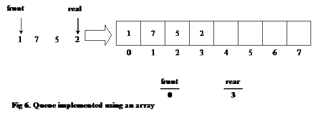
clip_image005
In the above figure, queue implementation using array is shown. As the array size is 8, therefore, the index of the array will be from 0 to 7. The number of elements inside array are 1, 7, 5 and 2, placed at start of the array. The front and rear in this implementation are not pointers but just indexes of arrays. front contains the starting index i.e. 0 while rear comprises 3.
Let’s see, how the enqueue() works:
clip_image006
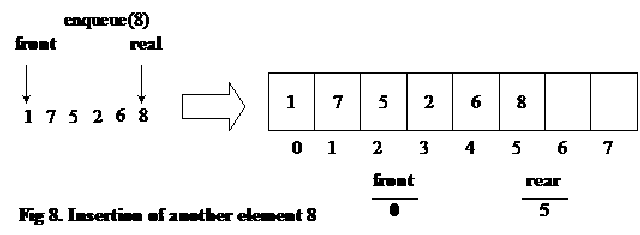
As shown in the above diagram, an element i.e. 6 has been inserted in the queue. Now, the rear index is containing 4 while the front has the same 0 index. Let’s see the figure of the array when another element 8 is inserted in the queue.
clip_image007
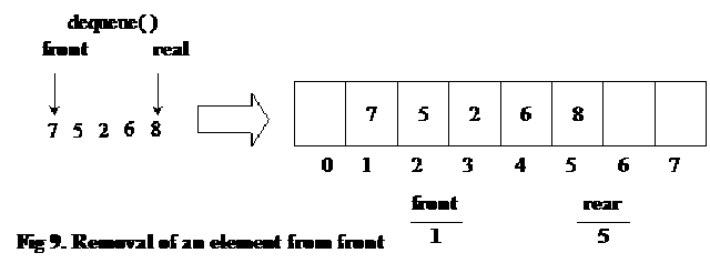
When an element is removed from the queue. It is removed from the front index.
clip_image008
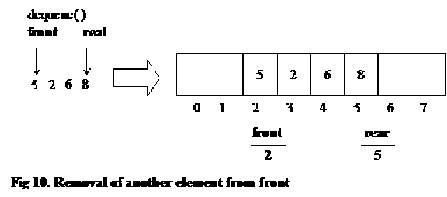
After another call of dequeue() function:
clip_image009
With the removal of element from the queue, we are not shifting the array elements. The shifting of elements might be an expensive exercise to perform and the cost is increased with the increase in number of elements in the array. Therefore, we will leave them as it is.
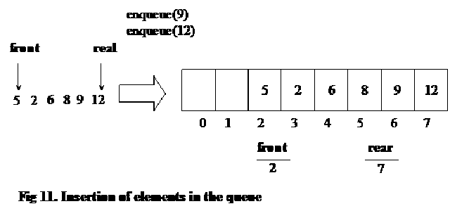
clip_image010
After insertion of two elements in the queue, the array that was used to implement it, has reached its limit as the last location of the array is in use now. We know that there is some problem with the array after it attained the size limit. We observed the similar problem while implementing a stack with the help of an array.
We can also see that two locations at the start of the array are vacant. Therefore, we should can consider how to use those locations appropriately in to insert more elements in the array.
Although, we have insert and removal operations running in constantly, yet we created a new problem that we cannot insert new elements even though there are two places available at the start of the array. The solution to this problem lies in allowing the queue to wrap around.
How can we wrap around? We can use circular array to implement the queue. We know how to make a linked list circular using pointers. Now we will see how can we make a circular array.
clip_image011
The number of locations in the above circular array are also eight, starting from index 0 to index 7. The index numbers are written outside the circle incremented in the clock-wise direction. To insert an element 21 in the array , we insert this element in the location, which is next to index 7.
clip_image012
Now, we will have to maintain four variables. front has the same index 2 while the, size is 8. ‘ rear’ has moved to index 0 and noElements is 7. Now, we can see that rear index has decreased instread of increasing. It has moved from index 7 to 0. front is containing index 2 i.e. higher than the index in rear. Let’ see, how do we implement the enqueue() method.
void enqueue( int x)
{
1. rear = (rear + 1) % size;
2. array[rear] = x;
3. noElements = noElements + 1;
}
In line 1 of the code, 1 is added in rear and the mod operator (that results in remainder of the two operands) is applied with size variable. This expression on the right of assignment in line 1 can result from 0 to 7 as size is containing value 8. This operator ensures that value of this expression will always be from 0 to 7 and increase or decrease from this. This resultant is assigned to the rear variable.
In line 2, the x (the value passed to enqueue() method to insert in the queue) is inserted in the array at the rear index position. Therefore, in the above case, the new element 21 is inserted at index 0 in the array.
In line 3, noElements is added to accumulate another element in the queue.
Let’s add another element in the queue.
clip_image013
Now, the queue, rather the array has become full. It is important to understand, that queue does not have such characteristic to become full. Only its implementation array has become full. To resolve this problem, we can use linked list to implement a queue. For the moment, while working with array, we will write the method isFull(), to determine the fullness of the array.
int isFull()
{
return noElements == size;
}
int isEmpty()
{
return noElements == 0;
}
isFull() returns true if the number of elements (noElements) in the array is equal to the size of the array. Otherwise, it returns false. It is the responsibility of the caller of the queue structure to call isFull() function to confirm that there is some space left in the queue to enqueue() more elements.
Similarly isEmpty() looks at the number of elements (noElements) in the queue. If there is no element, it returns true or vice versa..
Let’s see the dequeue() method.
clip_image014
int dequeue()
{
int x = array[front];
front = (front + 1) % size;
noElements = noElements - 1;
return x;
}
In the first line, we take out an element from the array at front index position and store it in a variable x. In the second line, front is incremented by 1 but as the array is circular, the index is looped from 0 to 7. That is why the mod (%) is being used. In the third line, number of elements (noElements) is reduced by 1 and finally the saved array element is returned.

C program to Read From a File

#include <stdio.h> #include <stdlib.h> void main() {     FILE *fptr;     char filename[15];     char ch;   ...