Quick Sort

 

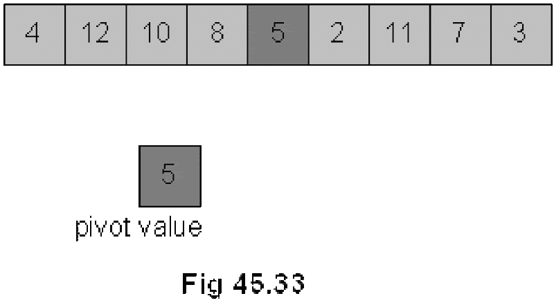
Quicksort is another divide and conquer algorithm. Quicksort is based on the idea of partitioning (splitting) the list around a pivot or split value. Quicksort is also a divide and conquer algorithm. We see pictorially, how the quick sort algorithm works. Suppose we have an array as shown in the figure Fig 45.33.

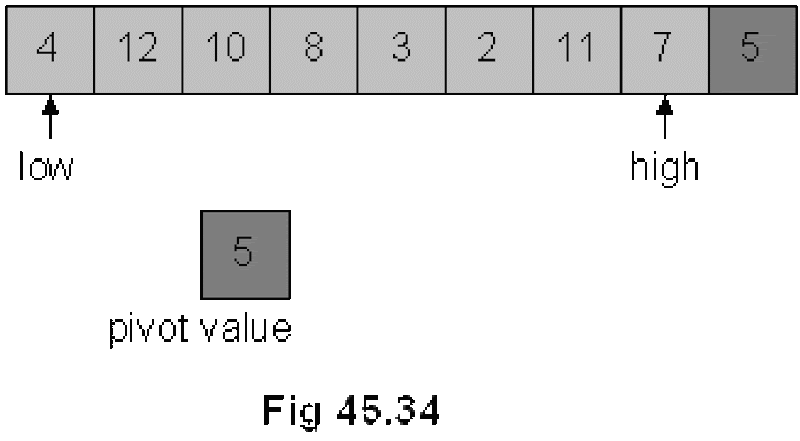
We select an element from the array and call it the pivot. In this array, the pivot is the middle element 5 of the array. Now, we swap this with the last element 3 of the array. The updated figure of the array is shown in Fig 45.34.

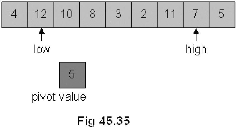
As shown in Fig 45.34, we used two indexes low and high. The index low is started from 0^th position of the array and goes towards right until n-1^th position. Inside this loop, an element that is bigger than the pivot is searched. The low index is incremented further as 4 is less than 5.

low is pointing to element 12 and it is stopped here as 12 is greater than 5. Now, we start from the other end, the high index is moved towards left from n-1^th position to 0. While coming from right to left, we search such an element that is smaller than 5. Elements 7 and 11 towards left are greater than 5, therefore, the high pointer is advanced further towards left. high index is stopped at the next position as next element 2 is smaller than 5. Following figure Fig 45.36 depicts the latest situation.

Divide and Conquer

We had started discussing three new sorting algorithms; merge sort, quick sort and heap sort. All of these three algorithms take time proportional to nlog₂n. Our elementary three sorting algorithms were taking n² time; therefore, these new algorithms with nlog₂n time are faster. In search operation, we were trying to reduce the time from n to log₂n.

Let’s discuss these sorting algorithms; merge sort, quick sort and heap sort in detail.

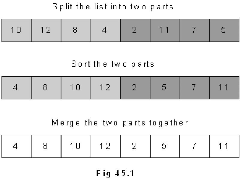
We had started our discussion from divide and conquer rule where we also saw an example. Instead of sorting a whole array, we will divide it in two parts, each part is sorted separately and then they are merged into a single array.

Let’ see few analysis to confirm the usefulness of the divide and conquer technique.

- To sort the halves approximate time is (n/2)2+(n/2)2

- To merge the two halves approximate time is n

- So, for n=100, divide and conquer takes approximately:

= (100/2)2 + (100/2)2 + 100

= 2500 + 2500 + 100

= 5100 (n2 = 10,000)

Comparison of Complexity of Algorithms

We have studied these three algorithms i.e. selection sort, insertion sort and bubble sort. Now considering the above three algorithms, we see that these algorithms are easy to understand. Coding for these algorithms is also easy. These three algorithms are in place algorithms. There is no need of extra storage for sorting an array by these algorithms. With respect to the time complexity, these algorithms are proportional to N². Here N is the number of elements. So we can see that as the value of N increases, the performance time of these algorithms increases considerably as it is proportional to N². Thus these algorithms are expensive with respect to time performance. There are algorithms that have the time complexity proportional to N log₂ (N). The following table shows the respective values of N² and N log₂(N) for some values of N.

N	N2	N Log2 (N)
10	100	33.21
100	10000	664.38
1000	1000000	9965.78
10000	100000000	132877.12
100000	10000000000	1660964.04
1000000	1E+12	19931568.57

From this table we can see that for a particular value of N, the value of N² is very large as compared to the value of N log₂ (N). Thus we see that the algorithms whose time complexity is proportional to N² are much time consuming as compared to the algorithms the time complexity of which is proportional to N log₂ (N). Thus we see that the N log₂ (N) algorithms are better than the N² algorithms.

N log₂ (N) Algorithms

Now let’s see the algorithms that are N log₂ (N) algorithms. These include the following algorithms.

• Merge Sort
• Quick Sort
• Heap Sort

These three algorithms fall under ‘divide and conquer category’. The divide and conquer strategy is well known in wars. The philosophy of this strategy is ,’ divide your enemy into parts and then conquer these parts’. To conquer these parts is easy, as these parts cannot resist or react like a big united enemy. The same philosophy is applied in the above algorithms. To understand the divide and conquer strategy in sorting algorithm, let’s consider an example. Suppose we have an unsorted array of numbers is given below.

Bubble Sort

The third sorting algorithm is bubble sort. The basic idea of this algorithm is that we bring the smaller elements upward in the array step by step and as a result, the larger elements go downward. If we think about array as a vertical one, we do bubble sort. The smaller elements come upward and the larger elements go downward in the array. Thus it seems a bubbling phenomenon. Due to this bubbling nature, this is called the bubble sort. Thus the basic idea is that the lighter bubbles (smaller numbers) rise to the top. This is for the sorting in ascending order. We can do this in the reverse order for the descending order.

The steps in the bubble sort can be described as below

• Exchange neighboring items until the largest item reaches the end of the array

• Repeat the above step for the rest of the array

In this sort algorithm, we do not search the array for the smallest number like in the other two algorithms. Also we do not insert the element by shifting the other elements. In this algorithm, we do pair-wise swapping. We will take first the elements and swap the smaller with the larger number. Then we do the swap between the next pair. By repeating this process, the larger number will be going to the end of the array and smaller elements come to the start of the array.

Insertion Sort

The main idea of insertion sort is

• Start by considering the first two elements of the array data. If found out of order, swap them

• Consider the third element; insert it into the proper position among the first three elements.

• Consider the fourth element; insert it into the proper position among the first four elements.

• … …

This algorithm is not something uncommon to the persons who know card playing. In the game of cards, a player gets 13 cards. He keeps them in the sorted order in his hand for his ease. A player looks at the first two cards, sorts them and keeps the smaller card first and then the second. Suppose that two cards were 9 and 8, the player swap them and keep 8 before 9. Now he takes the third card. Suppose, it is 10, then it is in its position. If this card is of number 2, the player will pick it up and put it on the start of the cards. Then he looks at the fourth card and inserts it in the first three cards (that he has sorted) at a proper place. He repeats the same process with all the cards and finally gets the cards in a sorted order. Thus in this algorithm, we keep the left part of the array sorted and take element from the right and insert it in the left part at its proper place. Due to this process of insertion, it is called insertion sorting.

Selection Sort

 

Suppose we have an array with different numbers. For sorting it in an ascending order, selection sorting will be applied on it in the following manner. We find the smallest number in the array and bring it to the position 1. We do the same process with the remaining part of the array and bring the smallest number among the remaining array to the next position. This process continues till the time all the positions of the array are filled with the elements. Thus the main idea of selection sort is that

• find the smallest element

• put it in the first position

• find the next smallest element in the remaining elements

• put it in the second position

• …

• And so on, until we get to the end of the array

Let’s understand this algorithm by considering an example with the help of figures.

Consider an array that has four numbers i.e. 19, 5, 7 and 12 respectively. Now we want to sort this array in ascending order. To sort the array, selection algorithm will be applied on it.

Binary Search

 

The binary search is an algorithm of searching, used with the sorted data. As we have sorted elements in the array, binary search method can be employed to find data in the array. The binary search finds an element in the sorted array in log n time. If we have 100000 elements in the array, the log 1000000 will be 20 i.e. very small as compared to 100000. Thus binary search is very fast.

The binary search is like looking up a phone number in the directory or looking up a word in the dictionary. For looking a word in the dictionary, we start from the middle in the dictionary. If the word that we are looking for comes before words on the page, it shows that the word should be before this page. So we look in the first half. Otherwise, we search for the word in the second half of the dictionary. Suppose the word is in the first half of the dictionary, we consider first half for looking the word. We have no need to look into the second half of the dictionary. Thus the data to be searched becomes half in a step. Now we divide this portion into two halves and look for the word. Here we again come to know that the word is in the first half or in the second half of this portion. The same step is repeated with the part that contains the required word. Finally, we come to the page where the required word exists. We see that in the binary search, the data to be searched becomes half in each step. And we find the entry very fast. The number of maximum steps needed to find an entry is log n, where n is the total number of entries. Now if we have 100000 entries, the maximum number of attempts (steps) required to find out the entry will be 20 (i.e. log 1000000).

If already sorted data is available, then it is better to apply an algorithm of binary search for finding some item inside instead of searching from start to the end in sequence. The application of this algorithm will help get the results very quickly.